Quant Basics 8: Bootstrapping and Response Surface
In the last section we investigated how the strategies we’ve selected from our train-test cluster were distributed in the parameter plot. We saw that they form a dense cluster in that plot which indicates that the PnL’s we see are not a result of overfitting since we would expect them to be more randomly distributed.
In this section we have a look at how to do a Monte-Carlo analysis of our PnL curve. All we do here is to draw random return samples from our curve and re-asseble them in a set of new PnL curves. The shortfall we see will give us some indication on how consistent our results are. This is particularly important as we want to avoid the possibility of large drawdowns.
def bootstrap(pnls,params,tickers,start,end,backend='file'):

    # Get the PnLs of our top strategies
    p = prices(tickers,start,end,backend=backend)
    best_params = get_best_parameters(params,pnls,50)
    pnl = calc_pnl(calc_signals(tickers,p,min(best_params[0]),max(best_params[1])),p)

    # Calculate the returns
    rets = np.diff(pnl)
    rets = rets[~np.isnan(rets)]
    last = []
    for i in range(500):

        # Random sampling step
        k = np.random.choice(rets,len(rets))
        ps = np.cumsum(k)
        if ~np.isnan(ps[-1]):
            last.append(ps[-1])

        # Plot the sample
        plt.subplot(211)
        plt.plot(ps)
        plt.xlabel('time')
        plt.ylabel('PnL')
    print 'actual pnl:',np.cumsum(rets)[-1],' bootstrapped mean pnl: ',np.nanmean(last)

    # Plot the distribution
    plt.subplot(212)
    plt.hist(last,30)
    plt.xlabel('PnL')
    plt.ylabel('N')
    plt.show()
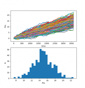
actual pnl: 14.9704493607 bootstrapped mean pnl: 14.9525417379
We can see that the mean PnL of the bootstrap is very close to the actual PnL of our strategy. That is a very encouraging result. The main issue usually arises when we have some extreme returns in our PnL curve that may skew our distribution. If this was the case we would need to be much more cautious to trade such a strategy unless we have a very good explanation for such returns.
The results of the bootstrap are shown below. On the top we see all the randomly sampled PnL curves and on the bottom show the distribution of the final PnLs of all these curves.
Here we’ve seen another way to assess our strategy. In the next section we will look at the response surface of the strategy with respect to the parameters. What we hope to see is a reasonably continuous surface, which tells us that our returns are not just due to some lucky coincidences.
The code base for this section can be found on Github.