Breaking the Sharpe ratio
by Qian Zhu and Tom Starke
If you want to learn about things deeply, you need to break them. Sharpe Ratio is one of the top metrics used by traders and investors to evaluate their trading strategy/investment systems. It is often referred to as the ‘risk-adjusted performance measures’, which gives confidence to investors by comparing the portfolio to a risk-free benchmark.
The Sharpe ratio is calculated as follows,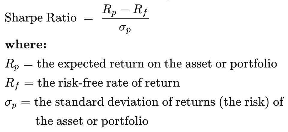 However, as we will see in the following sections, it can be ambiguous and may lead to misleading interpretations—the consequence of which may seriously impact our trading capital. To demonstrate this, let us look at a simple Buy and Hold strategy for a portfolio consisting of the e-commerce giant Amazon as the single asset. The trading strategy consists of the following logic:
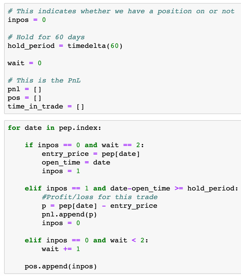
- start buying at Day 3;
- exit after holding for 60 days;
- wait for 2 days before trading again;
- repeat.
To execute this in Python, the first step is to download the price data: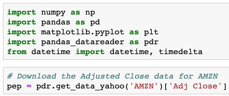
Next, we construct our backtest:
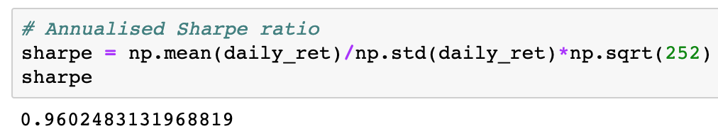
Time to calculate the Sharpe ratio! But before we do that, we need to calculate the daily return of our strategy. This can be achieved by the daily percentage change of price multiply by the pos array (denoting whether we have a position or not each day):
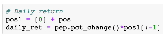
Note the manipulation of the pos array, so that we are multiplying the correct position with the daily percentage change of price. Now we can calculate the Sharpe ratio, which is about 0.96 for our strategy:
Profit per trade
Here comes the twist. Let’s have a look at the profit per trade — in two ways. One is the original profit per trade (as the trade happens according to our strategy); the other way is by sorting the profit per trade. Here’s the plot: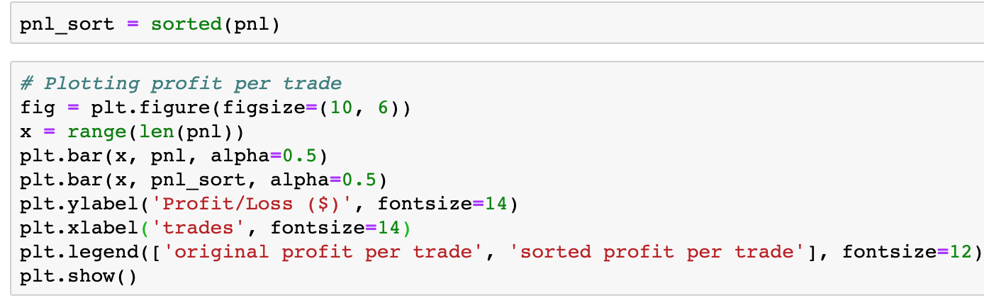
 Note that by sorting the profit per trade, we are simulating changing the order of the sequence of trades — from the largest losing trades to profitable trades. At this point, I invite you to pause and answer the following questions:
By changing the sequence of trades —
- Has the mean and standard deviation changed?
- Has the probability distribution changed?
- Has the Sharpe ratio changed? Is it still approximately 0.96 as we calculated above?
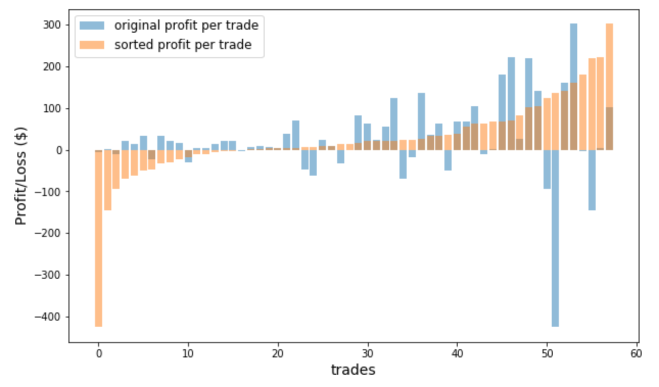
With your answers in mind, now we plot the cumulative P&L curve, which is one of the foremost important measures traders take to evaluate their trades.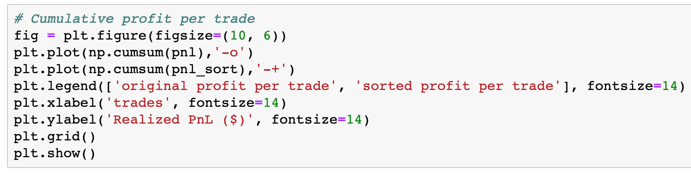
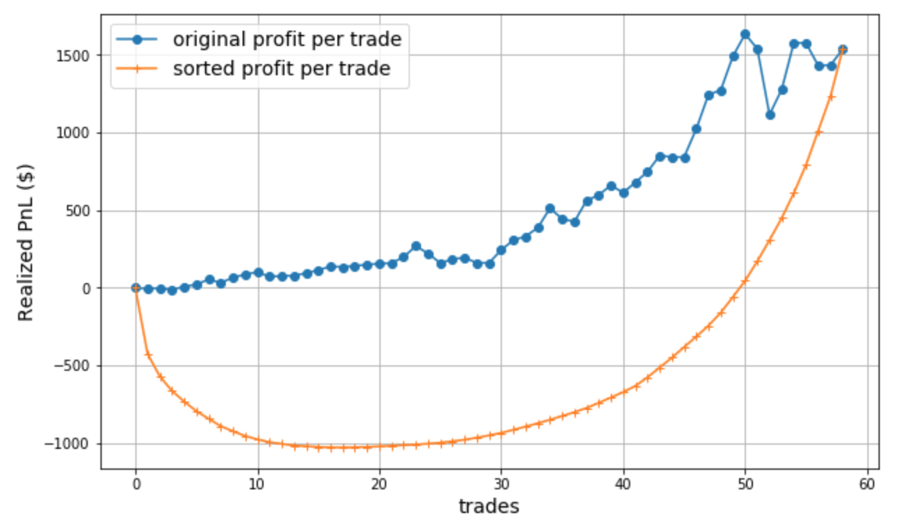 Surprise surprise! Why did we get two completely different curves? The curve from the sorted sequence (orange curve) showed we lost $1000 for quite some number of trades and only started climbing back out of the losing trades towards the end; whereas the other curve showed that we never lost any money from our original capital!
From the standpoint of a physicist/scientist, the two curves represent two different processes in terms of thermodynamics and information theory. The blue curve represents a Markov process, where the sequence of the P&L is more or less random in nature (the outcome of each trade depends on its own current state, i.e., the underlying price movements of this particular stock and the broader market conditions at a particular point in time). In comparison, the orange curve represents a perfectly ordered system from small to large, in other words, we can say that the outcome or state of a particular trade depends on the state of the previous trade. According to the laws of thermodynamics, two curves have different levels of entropy.
Shannon Entropy
We can also look at this from an information theorist’s perspective, using information entropy, introduced by Claude Shannon in his 1948 paper “A Mathematical Theory of Communication”. Basically, Shannon Entropy measures the degree of disorder or information contained in a data communication system. In financial markets, we can see direct analogue to this. Most of the time the financial data consists of random noise, and in some situations the data is not completely random but contains some degree of predictability—this is when traders/investors can capitalise on the predictability and survive. Specifically, Shannon Entropy (H) is defined by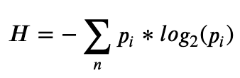 where ? is the number of possible outcomes, and ?? is the probability of the ??ℎ outcome occurring.
To calculate the Shannon Entropy for our P&L curves, we need to first convert the data into binary form (c.f. binary bits in a communications system). We are interested in the direction of the movement in the curve, so the pseudo code goes like this:
if current value > previous value:
Assign 1
else:
Assign 0
Let’s start with the easy case—the orange curve. Since the data points in this curve are ordered, we will be assigning 1 to all points, i.e., ?? will always be 1, as we are certain that every time the next data point will be greater than the current data point. Log of 1 is zero! So Shannon Entropy for this curve is 0.
How about another extreme case, where the movement of each data point is completely random? This represents a perfectly efficient market scenario. This is also easy to calculate, as ?? will always be 0.5. The Shannon Entropy for this case is reduced to H = -n*0.5*log2(0.5), which is 29 for our case where n = 58. This is the maximum entropy we would have for our trading data points.
For the blue curve, which is the actual P&L we had for the trading strategy, the Shannon Entropy will be somewhere between 0 and 29. This is because the probability for the direction of movement for each trade is neither 1 (we are totally certain) nor 0.5 (the process is completely random), but somewhere in between — a real scenario in practice. Of course, the smaller the entropy, the more certain we are with our trades and more likely to have a profitable strategy.
You may find this entropy concept perplexing, but what is more perplexing is when we look back at the questions we asked earlier — the answer to all three questions is NO. The blue and orange curves have the same Sharpe ratio, mean and standard deviation, and statistical distribution!
Do you now see the problem? Completely different systems (with different entropies) can have the same Sharpe ratio, as demonstrated above. This is due to the fact that Sharpe ratio only relies on capturing the standard deviation of the trades, i.e., volatility. Note that volatility does not equal risk. And the standard deviation is independent of the order of data points. From our example above, one might suffer substantial loss in the process, all of which is not revealed by the Sharpe ratio.
Comparing Bitcoin and S&P500
To illustrate the concepts further, let’s investigate two very different instruments — Bitcoin and the S&P500 index. The figure below tells the price stories for the two instruments between late 2015 and January 2020. One can see that (not surprisingly) Bitcoin has higher volatility than S&P500, especially around 2018 — anyone holding Bitcoin at that time would need to have a mind of steel to withstand the roller coaster behaviours. 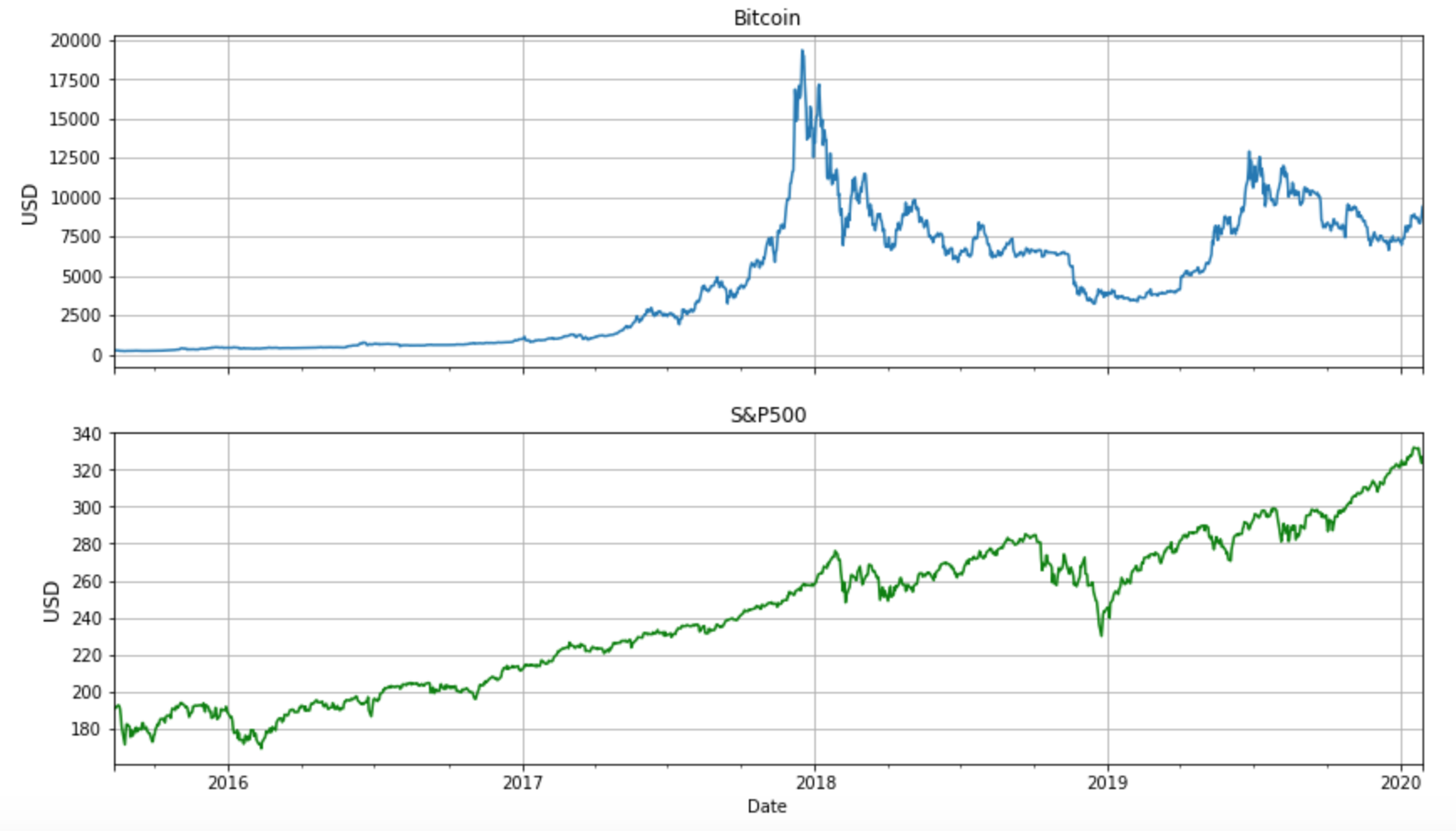 We are interested to see the Sharpe ratios for these two instruments. To do so, let’s run a backtest for both Bitcoin and S&P500 implementing the simple Buy and Hold strategy mentioned above. The full Python Jupyter notebook can be found here. The resulting annualised Sharpe ratios are shown in Table 1. If judging purely from the Sharpe ratio, Bitcoin is a better investment as it has a higher Sharpe ratio than the S&P500. However, looking back at the price curves, Bitcoin went through a bubble bursting phase in 2018 — the Bitcoin price dropped 80% from its highest point! This is a dramatic drawdown from the original capital. All this was not reflected in the Sharpe ratio.
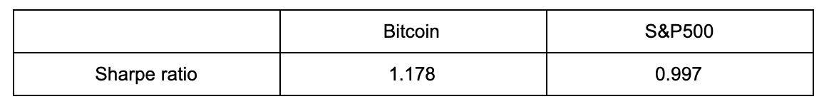 Table 1. Sharpe ratios calculated for Bitcoin and S&P500 implementing the simple Buy and Hold strategy.
Conclusion
As traders or investors we need to evaluate our trading strategy using a rigorous approach, at least not relying on a single performance metric alone. As we have seen in this article, different investment systems (e.g., with different underlying mechanisms, or entropies, or price drawdowns) may have the same Sharpe ratios. If one is not performing the due diligence or cross checking, the original trading capital may easily suffer. Furthermore, knowing the limitation of individual performance metric and looking at the problem from different angles may sometimes save us from dangerous (aka capital-wiping) situations.