Kdb+ vs. Python
What is kdb+?
Kdb+ is a powerful column based time series database. It is commonly used in investment banks and hedge funds around the world for extremely fast time series analysis.
Kdb+ uses vector language Q, which itself was built for speed and expressiveness. Q commands can be entered straight into the console, as compilation is not needed. The terms Q and Kdb+ are usually used interchangeably.
What makes kdb+ fast is that is column-oriented, and in-memory. Column-oriented means each column of data is stored sequentially. With regards to time series data, analysis is performed on columns e.g. coding up a function that can find the average price from certain trades. Row-oriented databases are much slower at this as they would need to read across each record one by one. In memory means the data is stored in RAM. This has been made possible with technological advancements in servers.
In this blog post I will time a linear regression in q and compare its performance to the same regression coded in Python. Each step and parameters in the linear regressions are matched for a fair comparison between Python and Q.
Installing Kdb+
To follow along, you can install the 32 bit version of kdb+. This version is free to use and can be set up in just a few steps. Note I am using Mac OSX.
- Download kdb+ at https://kx.com/download/
- Copy the q folder from Downloads into the home directory.
- In the terminal type
vi ~/.profile
- Use vi to add the following code to your .profile file, which can be found in your home directory. Type :wq to save and exit the file after the code.
export QHome=~/q

export PATH=$PATH:$QHOME/m32
- Use the source command to load these variables into your current session (you only have to do this once).
Source ~/.profile
- Type q to enter a q session. Type \\ to exit.
Linear Regression in kdb+
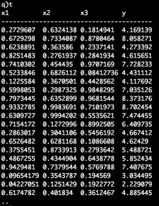
In the example script below, we generate 1,200,300 random data records for the table. The table t is initialised with floating type integers, and x1, x2, x3 parameters as columns. We update the table t by appending the column y. The ys in this column are computed from the regression equation y = 1 + (2*x1) + (3*x2) + (4*x3). The independent (x) and dependent (y) variables are assigned to ind and dep. Finally we compute out the regression parameters. enlist returns arguments in a list.
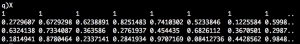
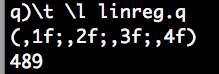
n:1200300; t:([]x1:n?1f;x2:n?1f;x3:n?1f)

update y:1+(2*x1)+(3*x2)+(4*x3) from `t;

indx:`x1`x2`x3

depy:enlist`y

X:enlist[count[t]#1f],t indx

inv[X mmu flip X] mmu X mmu flip t depy
The following code times code execution in q. The regression took only 489 milliseconds to execute. And as expected, x1, x2 and x3 (the “coefficients” of the regression) are 1, 2, 3 and 4.
Linear Regression in Python
The equivalent of the above example in Python:
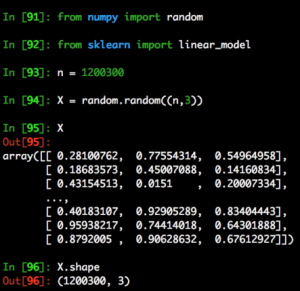
from numpy import random

from sklearn import linear_model

n = 1200300

X = random.random((n,3))

y = 1+2*X[:,0]+3*X[:,1]+4*X[:,2]

y = y[:,None]

reg = linear_model.linearRegression()

reg.fit(X,y)

print(reg.intercept_,reg.coef_)
Let’s break the python script down to see how it replicates the q code.
We first generate a 2D array with random values between 0 and 1. Like the table we generated in q, it has 1200300 rows and 3 columns.
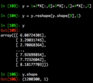
Next we calculate values for y. Like the example in q, we compute y by multiplying 2,3,4 with X’s columns respectively. X[:,0] extracts the first column, X[:,1] extracts the second column, etc. We do need to reshape it with y[:,None] because of the dimension requirements by sklearn. (target y must be a numpy array of shape [n_samples, n_targets])
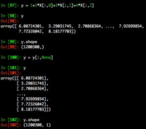
For those not familiar with y[:,None] it is the same as using the reshape function like so.
We then initialise the linear regression model, fit to our data and print the intercept and regression coefficients.
reg = linear_model.linearRegression()

reg.fit(X,y)

linearRegression(copy_I=True, fit_intercept=True, n_jobs=1, normalize=False)

print(reg.intercept_,reg.coef_)
The output is [1.][[2. 3. 4.]]
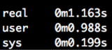
Running time python linreg.py gives us an execution time of 1.163s.
You can read more about what real, user and sys mean here
Kdb+ is the clear winner when it comes to speed of Big Data analysis. For those not yet willing to give up Python completely, you will be glad to hear there exists a Python & q interface, PyQ. PyQ provides seamless integration of Python and q code. I will discuss this in future kdb+ posts.